2004-(II)-Dynamic light scattering
Article Index
Data evaluation of dynamic light scattering:
The central quantity of the evaluation of correlation spectroscopy is the decay time also named the correlation-time τ. Unfortunately, it is not possible to detect this frequency with classical optical methods. As a consequence, it is substantial to use optical mixing techniques, like homogenous mixing, heterogenous mixing (homodyne and heterodyne techniques) and the self-beating method.
Self-beating spectroscopy:
The principle of self-beating spectroscopy is based on mixing of scattered light with the original light on analyzing the resulting signal with low-frequency intermediate signal. This is realized in three steps:
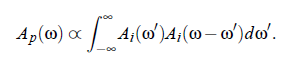
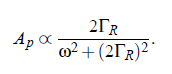
Consider a signal of field strength E (R ,ω) with spectrum A , that has to be shifted into the lower frequencies. This happens with the aid of a local-oscillator signal. After this mixing procedure, it is possible to describe the scattered light with the help of convolution integral of the incoming spectrum (Ap , spectrum of the photon flux):
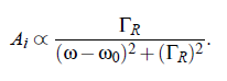
On the one side, the photon flux i(t ) is proportional to the light intensity, |I (ω)| = |E (ω)|^2 . On the other side, the considered Rayleigh line is of the shape of a Lorentz curve, with the the half-bandwidth ΓR and the center frequency ω_0:
For simple fluids the half-bandwidth ΓR (see Fig.(3.16)) of the Lorenz-curve can be represented by:
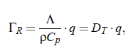
here denotes D_T the thermal diffusivity, Λ the thermal conductivity, ρ the density, C, the heat capacity at constant pressure p as well as q, the amount of the scattering vector. The next step is to find a tool to measure the spectrum. This can be realized with the aid of Correlation Spectroscopy.
Correlation Spectroscopy: The Wiener-Khinchin theorem |Af (ω)| = F Φ [f (t )] relates the signal f (t ) with the amount of the spectrum Af (ω). Here is F −1 the inverse Fouriertransform and Φ [f (t )] is the autocorrelation function of f(t). As mentioned before, the signal i(t) of the photon flux is proportional to the light intensity I (t). Practically, in an experiment the autocorrelation function Φ [i], which is proportional to the autocorrelation function of Φ [I ], is determined. Consequently, the following expression results:
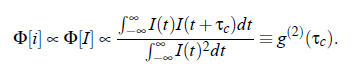
In an experiment the interest is not focused on the intensity spectrum of the but in the spectrum of electric filed E (t ). Due to the well known relation I (t ) = |E (t )| , the expression (3.23) for the electric field is given by:
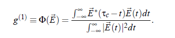
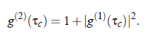
Finally, the autocorrelation function g (2) of the intensity I (t ) and the autocorrelation function g (1) of the field E (t) are related by the so-called Siegert relation:
In the DLS experiment one has to do with the Lorentz profile. The autocorrelation function of this profile is given by:
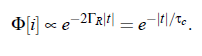
This equation allows to determine the half-with ΓR of Rayleigh-line from the correlation-time 1/2ΓR of the photon autocorrelation function.
Photon statistics: All considerations have been done with the assumption that i(t ) ∝ I (t ). In principle, this can be done for sufficiently high scattering count rates. For experiments with lower rates it is substantial to use adequate statistics.